OpenVINO™ を使用した単眼による視覚慣性深度の推定
この Jupyter ノートブックは、ローカルへのインストール後にのみ起動できます。

全体的な方法論。VI-Depth リポジトリーから取得した図表。
著者は、単眼深度推定と視覚慣性オドメトリーを統合して、メートル法スケールの高密度深度推定値を生成する視覚慣性深度推定パイプラインを発表しました。このアプローチは 3 つのステージで構成されます。
入力処理では、RGBと慣性計測ユニット (IMU) のデータが視覚慣性オドメトリーとともに単眼深度推定に入力されます。
グローバルスケールとシフト・アライメントでは、単眼深度推定値が視覚慣性オドメトリー (VIO) からのスパース深度に最小二乗法で適合されます。
学習ベースの稠密スケール・アライメントでは、グローバルにアライメントされた深度が、ScaleMapLearner (SML) によって回帰された稠密スケールマップを使用してローカルに再アライメントされます。
上の図の下部にある画像は、パイプラインで処理されている Visual Odometry with Inertial and Depth (VOID) サンプルを示しています。左から右に、入力 RGB、グラウンドトゥルース深度、VIO からのスパース深度、グローバルに調整された深度、スケール・マップ・スキャフォールディング、SML によって回帰された高密度スケールマップ、最終的な深度出力です。
画像パイプラインによって処理される VOID サンプルの図。VI-Depth リポジトリーから取得した画像。
前処理、モデル変換、基本ユーティリティー・コードについては、VI-Depth リポジトリーを参照してください。その一部はすでに utils ディレクトリーにそのまま保存されています。同時に、異なる形式のモデルを別の形式を介して標準の OpenVINO™ IR モデル表現に変換するモデル変換を実行する方法も学習します。
目次
インポート
# Import sys beforehand to inform of Python version <= 3.7 not being supported
import sys

if sys.version_info.minor < 8:
    print('Python3.7 is not supported. Some features might not work as expected')

# Download the correct version of the PyTorch deep learning library associated with image models
# alongside the lightning module
%pip uninstall -q -y openvino-dev openvino openvino-nightly
%pip install -q --extra-index-url https://download.pytorch.org/whl/cpu "pytorch-lightning" "timm>=0.6.12" "openvino-nightly"
Note: you may need to restart the kernel to use updated packages.
DEPRECATION: pytorch-lightning 1.6.5 has a non-standard dependency specifier torch>=1.8.*. pip 24.1 will enforce this behaviour change. A possible replacement is to upgrade to a newer version of pytorch-lightning or contact the author to suggest that they release a version with a conforming dependency specifiers. Discussion can be found at https://github.com/pypa/pip/issues/12063
ERROR: pip's dependency resolver does not currently take into account all the packages that are installed. This behaviour is the source of the following dependency conflicts.
googleapis-common-protos 1.62.0 requires protobuf!=3.20.0,!=3.20.1,!=4.21.1,!=4.21.2,!=4.21.3,!=4.21.4,!=4.21.5,<5.0.0.dev0,>=3.19.5, but you have protobuf 3.20.1 which is incompatible.
onnx 1.15.0 requires protobuf>=3.20.2, but you have protobuf 3.20.1 which is incompatible.
paddlepaddle 2.6.0 requires protobuf>=3.20.2; platform_system != "Windows", but you have protobuf 3.20.1 which is incompatible.
tensorflow 2.12.0 requires protobuf!=4.21.0,!=4.21.1,!=4.21.2,!=4.21.3,!=4.21.4,!=4.21.5,<5.0.0dev,>=3.20.3, but you have protobuf 3.20.1 which is incompatible.
tensorflow-metadata 1.14.0 requires protobuf<4.21,>=3.20.3, but you have protobuf 3.20.1 which is incompatible.
Note: you may need to restart the kernel to use updated packages.
import matplotlib.pyplot as plt
import matplotlib.image as mpimg
import numpy as np
import openvino as ov
import torch
import torchvision
from pathlib import Path
from shutil import rmtree
from typing import Optional, Tuple

sys.path.append('../utils')
from notebook_utils import download_file

sys.path.append('vi_depth_utils')
import data_loader
import modules.midas.transforms as transforms
import modules.midas.utils as utils
from modules.estimator import LeastSquaresEstimator
from modules.interpolator import Interpolator2D
from modules.midas.midas_net_custom import MidasNet_small_videpth
# Ability to display images inline
%matplotlib inline
モデルとチェックポイントの読み込み
ここでの完全なパイプラインには、深度推定用のモデルと、高密度スケールマップの回帰を担当する ScaleMapLearner モデルの 2 つのモデルのみが必要です。オリジナルの VI-Depth リポジトリーで提供されているモデルの表が、ユーザーがダウンロードできるようにそのまま提示されています。VOID は、これらのモデルがトレーニングされた元のデータセットの名前です。VOID の後の数字は、密度マップの \(150\)、\(500\)、および \(1500\) レベルに対応するスパース密マップのサンプルをトレーニングした後に取得されたモデル内のチェックポイントを表します。ハイライト表示されたリンクのいずれかを右クリックし、“Copy link address” をクリックするだけです。次のセルのこのリンクを使用して、ScaleMapLearner モデルをダウンロードします。興味深いことに、ご覧のとおり、ScaleMapLearner が深度予測モデルを決定します。
深度予測 |
VOID 150 の SML |
VOID 500 の SML |
VOID 1500 の SML |
|---|---|---|---|
DPT-BEiT-Large |
|||
DPT-SwinV2-Large |
|||
DPT-Large |
|||
DPT-Hybrid |
モデル* |
||
DPT-SwinV2-Tiny |
|||
DPT-LeViT |
|||
MiDaS-small |
*TartanAir の事前トレーニングも利用可能: モデル
# Base directory in which models would be stored as a pathlib.Path variable
MODEL_DIR = Path('model')

# Mapping between depth predictors and the corresponding scale map learners
PREDICTOR_MODEL_MAP = {'dpt_beit_large_512': 'DPT_BEiT_L_512',
                       'dpt_swin2_large_384': 'DPT_SwinV2_L_384',
                       'dpt_large': 'DPT_Large',
                       'dpt_hybrid': 'DPT_Hybrid',
                       'dpt_swin2_tiny_256': 'DPT_SwinV2_T_256',
                       'dpt_levit_224': 'DPT_LeViT_224',
                       'midas_small': 'MiDaS_small'}
# Create the model directory adjacent to the notebook and suppress errors if the directory already exists
MODEL_DIR.mkdir(exist_ok=True)

# Here we will be downloading the SML model corresponding to the MiDaS-small depth predictor for
# the checkpoint captured after training on 1500 points of the density level. Suppress errors if the file already exists
download_file('https://github.com/isl-org/VI-Depth/releases/download/v1/sml_model.dpredictor.midas_small.nsamples.1500.ckpt', directory=MODEL_DIR, silent=True)

# Take a note of the samples. It would be of major use later on
NSAMPLES = 1500
model/sml_model.dpredictor.midas_small.nsamples.1500.ckpt: 0%| | 0.00/208M [00:00<?, ?B/s]
# Set the same model directory for downloading the depth predictor model which is available on
# PyTorch hub
torch.hub.set_dir(str(MODEL_DIR))


# A utility function for utilising the mapping between depth predictors and
# scale map learners so as to download the former
def get_model_for_predictor(depth_predictor: str, remote_repo: str = 'intel-isl/MiDaS') -> str:
    """
    Download a model from the pre-validated 'isl-org/MiDaS:2.1' set of releases on the GitHub repo
    while simultaneously trusting the repo permanently

    :param: depth_predictor: Any depth estimation model amongst the ones given at https://github.com/isl-org/VI-Depth#setup
    :param: remote_repo: The remote GitHub repo from where the models will be downloaded
    :returns: A PyTorch model callable
    """

    # Workaround for avoiding rate limit errors
    torch.hub._validate_not_a_forked_repo = lambda a, b, c: True

    return torch.hub.load(remote_repo, PREDICTOR_MODEL_MAP[depth_predictor], skip_validation=True, trust_repo=True)
# Execute the above function so as to download the MiDaS-small model
# and get the output of the model callable in return
depth_model = get_model_for_predictor('midas_small')
Downloading: "https://github.com/intel-isl/MiDaS/zipball/master" to model/master.zip
Loading weights: None
/opt/home/k8sworker/ci-ai/cibuilds/ov-notebook/OVNotebookOps-609/.workspace/scm/ov-notebook/.venv/lib/python3.8/site-packages/torch/hub.py:294: UserWarning: You are about to download and run code from an untrusted repository. In a future release, this won't be allowed. To add the repository to your trusted list, change the command to {calling_fn}(..., trust_repo=False) and a command prompt will appear asking for an explicit confirmation of trust, or load(..., trust_repo=True), which will assume that the prompt is to be answered with 'yes'. You can also use load(..., trust_repo='check') which will only prompt for confirmation if the repo is not already trusted. This will eventually be the default behaviour
  warnings.warn(
Downloading: "https://github.com/rwightman/gen-efficientnet-pytorch/zipball/master" to model/master.zip
Downloading: "https://github.com/rwightman/pytorch-image-models/releases/download/v0.1-weights/tf_efficientnet_lite3-b733e338.pth" to model/checkpoints/tf_efficientnet_lite3-b733e338.pth
Downloading: "https://github.com/isl-org/MiDaS/releases/download/v2_1/midas_v21_small_256.pt" to model/checkpoints/midas_v21_small_256.pt
0%| | 0.00/81.8M [00:00<?, ?B/s]
0%| | 320k/81.8M [00:00<00:27, 3.15MB/s]
1%| | 720k/81.8M [00:00<00:23, 3.68MB/s]
1%|▏ | 1.08M/81.8M [00:00<00:22, 3.78MB/s]
2%|▏ | 1.47M/81.8M [00:00<00:21, 3.88MB/s]
2%|▏ | 1.86M/81.8M [00:00<00:21, 3.83MB/s]
3%|▎ | 2.27M/81.8M [00:00<00:21, 3.95MB/s]
3%|▎ | 2.67M/81.8M [00:00<00:20, 4.05MB/s]
4%|▎ | 3.06M/81.8M [00:00<00:23, 3.55MB/s]
4%|▍ | 3.44M/81.8M [00:00<00:23, 3.53MB/s]
5%|▍ | 3.86M/81.8M [00:01<00:21, 3.76MB/s]
5%|▌ | 4.27M/81.8M [00:01<00:21, 3.84MB/s]
6%|▌ | 4.66M/81.8M [00:01<00:20, 3.90MB/s]
6%|▌ | 5.05M/81.8M [00:01<00:21, 3.81MB/s]
7%|▋ | 5.45M/81.8M [00:01<00:20, 3.94MB/s]
7%|▋ | 5.86M/81.8M [00:01<00:19, 4.03MB/s]
8%|▊ | 6.25M/81.8M [00:01<00:19, 4.01MB/s]
8%|▊ | 6.64M/81.8M [00:01<00:19, 4.02MB/s]
9%|▊ | 7.03M/81.8M [00:01<00:20, 3.89MB/s]
9%|▉ | 7.43M/81.8M [00:02<00:19, 3.97MB/s]
10%|▉ | 7.84M/81.8M [00:02<00:19, 4.07MB/s]
10%|█ | 8.23M/81.8M [00:02<00:19, 4.03MB/s]
11%|█ | 8.64M/81.8M [00:02<00:18, 4.05MB/s]
11%|█ | 9.03M/81.8M [00:02<00:19, 3.92MB/s]
12%|█▏ | 9.45M/81.8M [00:02<00:18, 4.06MB/s]
12%|█▏ | 9.84M/81.8M [00:02<00:18, 4.01MB/s]
13%|█▎ | 10.2M/81.8M [00:02<00:18, 4.05MB/s]
13%|█▎ | 10.6M/81.8M [00:02<00:19, 3.92MB/s]
13%|█▎ | 11.0M/81.8M [00:02<00:19, 3.86MB/s]
14%|█▍ | 11.4M/81.8M [00:03<00:18, 3.97MB/s]
14%|█▍ | 11.8M/81.8M [00:03<00:18, 4.04MB/s]
15%|█▍ | 12.2M/81.8M [00:03<00:17, 4.10MB/s]
15%|█▌ | 12.6M/81.8M [00:03<00:18, 3.99MB/s]
16%|█▌ | 13.0M/81.8M [00:03<00:18, 3.91MB/s]
16%|█▋ | 13.4M/81.8M [00:03<00:17, 4.01MB/s]
17%|█▋ | 13.8M/81.8M [00:03<00:17, 4.07MB/s]
17%|█▋ | 14.2M/81.8M [00:03<00:17, 4.11MB/s]
18%|█▊ | 14.6M/81.8M [00:03<00:18, 3.91MB/s]
18%|█▊ | 15.0M/81.8M [00:04<00:17, 3.98MB/s]
19%|█▉ | 15.5M/81.8M [00:04<00:17, 4.09MB/s]
19%|█▉ | 15.9M/81.8M [00:04<00:17, 3.91MB/s]
20%|█▉ | 16.2M/81.8M [00:04<00:17, 3.95MB/s]
20%|██ | 16.7M/81.8M [00:04<00:16, 4.03MB/s]
21%|██ | 17.1M/81.8M [00:04<00:16, 4.08MB/s]
21%|██▏ | 17.5M/81.8M [00:04<00:16, 4.02MB/s]
22%|██▏ | 17.9M/81.8M [00:04<00:17, 3.93MB/s]
22%|██▏ | 18.2M/81.8M [00:04<00:16, 3.96MB/s]
23%|██▎ | 18.7M/81.8M [00:04<00:16, 4.10MB/s]
23%|██▎ | 19.1M/81.8M [00:05<00:16, 4.04MB/s]
24%|██▍ | 19.5M/81.8M [00:05<00:16, 3.95MB/s]
24%|██▍ | 19.9M/81.8M [00:05<00:16, 3.97MB/s]
25%|██▍ | 20.2M/81.8M [00:05<00:16, 4.00MB/s]
25%|██▌ | 20.7M/81.8M [00:05<00:15, 4.07MB/s]
26%|██▌ | 21.1M/81.8M [00:05<00:16, 3.98MB/s]
26%|██▌ | 21.5M/81.8M [00:05<00:15, 3.97MB/s]
27%|██▋ | 21.9M/81.8M [00:05<00:15, 4.00MB/s]
27%|██▋ | 22.2M/81.8M [00:05<00:15, 4.02MB/s]
28%|██▊ | 22.7M/81.8M [00:06<00:15, 4.03MB/s]
28%|██▊ | 23.1M/81.8M [00:06<00:15, 3.99MB/s]
29%|██▊ | 23.5M/81.8M [00:06<00:15, 4.00MB/s]
29%|██▉ | 23.9M/81.8M [00:06<00:15, 4.04MB/s]
30%|██▉ | 24.3M/81.8M [00:06<00:14, 4.03MB/s]
30%|███ | 24.7M/81.8M [00:06<00:14, 4.04MB/s]
31%|███ | 25.1M/81.8M [00:06<00:14, 3.98MB/s]
31%|███ | 25.5M/81.8M [00:06<00:14, 3.99MB/s]
32%|███▏ | 25.9M/81.8M [00:06<00:14, 4.04MB/s]
32%|███▏ | 26.2M/81.8M [00:06<00:14, 4.06MB/s]
33%|███▎ | 26.6M/81.8M [00:07<00:14, 4.04MB/s]
33%|███▎ | 27.0M/81.8M [00:07<00:14, 4.04MB/s]
34%|███▎ | 27.4M/81.8M [00:07<00:14, 3.96MB/s]
34%|███▍ | 27.8M/81.8M [00:07<00:14, 3.96MB/s]
35%|███▍ | 28.2M/81.8M [00:07<00:13, 4.03MB/s]
35%|███▍ | 28.6M/81.8M [00:07<00:13, 4.03MB/s]
35%|███▌ | 29.0M/81.8M [00:07<00:13, 4.04MB/s]
36%|███▌ | 29.4M/81.8M [00:07<00:13, 4.04MB/s]
36%|███▋ | 29.8M/81.8M [00:07<00:13, 3.97MB/s]
37%|███▋ | 30.2M/81.8M [00:07<00:13, 3.98MB/s]
37%|███▋ | 30.6M/81.8M [00:08<00:13, 3.99MB/s]
38%|███▊ | 31.0M/81.8M [00:08<00:13, 4.02MB/s]
38%|███▊ | 31.4M/81.8M [00:08<00:13, 4.04MB/s]
39%|███▉ | 31.8M/81.8M [00:08<00:12, 4.04MB/s]
39%|███▉ | 32.1M/81.8M [00:08<00:13, 3.97MB/s]
40%|███▉ | 32.5M/81.8M [00:08<00:12, 3.99MB/s]
40%|████ | 32.9M/81.8M [00:08<00:12, 3.99MB/s]
41%|████ | 33.3M/81.8M [00:08<00:12, 4.06MB/s]
41%|████ | 33.7M/81.8M [00:08<00:12, 4.06MB/s]
42%|████▏ | 34.1M/81.8M [00:09<00:12, 3.99MB/s]
42%|████▏ | 34.5M/81.8M [00:09<00:12, 4.00MB/s]
43%|████▎ | 34.9M/81.8M [00:09<00:12, 3.99MB/s]
43%|████▎ | 35.3M/81.8M [00:09<00:12, 4.01MB/s]
44%|████▎ | 35.7M/81.8M [00:09<00:11, 4.07MB/s]
44%|████▍ | 36.1M/81.8M [00:09<00:11, 4.06MB/s]
45%|████▍ | 36.5M/81.8M [00:09<00:11, 4.05MB/s]
45%|████▌ | 36.9M/81.8M [00:09<00:11, 3.94MB/s]
46%|████▌ | 37.3M/81.8M [00:09<00:11, 3.98MB/s]
46%|████▌ | 37.7M/81.8M [00:09<00:11, 4.00MB/s]
47%|████▋ | 38.1M/81.8M [00:10<00:11, 4.07MB/s]
47%|████▋ | 38.5M/81.8M [00:10<00:11, 4.05MB/s]
47%|████▋ | 38.8M/81.8M [00:10<00:11, 4.04MB/s]
48%|████▊ | 39.2M/81.8M [00:10<00:11, 3.98MB/s]
48%|████▊ | 39.6M/81.8M [00:10<00:11, 3.98MB/s]
49%|████▉ | 40.0M/81.8M [00:10<00:11, 3.97MB/s]
49%|████▉ | 40.4M/81.8M [00:10<00:10, 4.03MB/s]
50%|████▉ | 40.8M/81.8M [00:10<00:10, 4.06MB/s]
50%|█████ | 41.2M/81.8M [00:10<00:10, 4.03MB/s]
51%|█████ | 41.6M/81.8M [00:10<00:10, 3.96MB/s]
51%|█████▏ | 42.0M/81.8M [00:11<00:10, 3.97MB/s]
52%|█████▏ | 42.4M/81.8M [00:11<00:10, 4.00MB/s]
52%|█████▏ | 42.8M/81.8M [00:11<00:10, 4.06MB/s]
53%|█████▎ | 43.2M/81.8M [00:11<00:09, 4.05MB/s]
53%|█████▎ | 43.6M/81.8M [00:11<00:09, 4.05MB/s]
54%|█████▎ | 44.0M/81.8M [00:11<00:09, 3.99MB/s]
54%|█████▍ | 44.3M/81.8M [00:11<00:09, 3.94MB/s]
55%|█████▍ | 44.8M/81.8M [00:11<00:09, 4.03MB/s]
55%|█████▌ | 45.2M/81.8M [00:11<00:09, 4.08MB/s]
56%|█████▌ | 45.5M/81.8M [00:11<00:09, 4.03MB/s]
56%|█████▌ | 45.9M/81.8M [00:12<00:09, 3.99MB/s]
57%|█████▋ | 46.3M/81.8M [00:12<00:09, 3.98MB/s]
57%|█████▋ | 46.7M/81.8M [00:12<00:09, 3.97MB/s]
58%|█████▊ | 47.1M/81.8M [00:12<00:08, 4.05MB/s]
58%|█████▊ | 47.5M/81.8M [00:12<00:08, 4.04MB/s]
59%|█████▊ | 47.9M/81.8M [00:12<00:08, 4.00MB/s]
59%|█████▉ | 48.3M/81.8M [00:12<00:08, 3.98MB/s]
60%|█████▉ | 48.7M/81.8M [00:12<00:08, 3.98MB/s]
60%|██████ | 49.1M/81.8M [00:12<00:08, 4.08MB/s]
61%|██████ | 49.5M/81.8M [00:13<00:08, 4.03MB/s]
61%|██████ | 49.9M/81.8M [00:13<00:08, 4.03MB/s]
61%|██████▏ | 50.3M/81.8M [00:13<00:08, 3.98MB/s]
62%|██████▏ | 50.7M/81.8M [00:13<00:08, 3.91MB/s]
62%|██████▏ | 51.1M/81.8M [00:13<00:08, 4.02MB/s]
63%|██████▎ | 51.5M/81.8M [00:13<00:07, 4.08MB/s]
63%|██████▎ | 51.9M/81.8M [00:13<00:07, 4.03MB/s]
64%|██████▍ | 52.3M/81.8M [00:13<00:07, 3.91MB/s]
64%|██████▍ | 52.7M/81.8M [00:13<00:07, 4.01MB/s]
65%|██████▍ | 53.1M/81.8M [00:13<00:07, 4.04MB/s]
65%|██████▌ | 53.5M/81.8M [00:14<00:07, 4.05MB/s]
66%|██████▌ | 53.9M/81.8M [00:14<00:07, 4.02MB/s]
66%|██████▋ | 54.3M/81.8M [00:14<00:07, 3.93MB/s]
67%|██████▋ | 54.7M/81.8M [00:14<00:07, 4.01MB/s]
67%|██████▋ | 55.1M/81.8M [00:14<00:06, 4.02MB/s]
68%|██████▊ | 55.5M/81.8M [00:14<00:06, 4.08MB/s]
68%|██████▊ | 55.9M/81.8M [00:14<00:06, 4.04MB/s]
69%|██████▉ | 56.3M/81.8M [00:14<00:06, 3.93MB/s]
69%|██████▉ | 56.7M/81.8M [00:14<00:06, 3.98MB/s]
70%|██████▉ | 57.1M/81.8M [00:14<00:06, 4.04MB/s]
70%|███████ | 57.5M/81.8M [00:15<00:06, 4.04MB/s]
71%|███████ | 57.9M/81.8M [00:15<00:06, 4.06MB/s]
71%|███████ | 58.3M/81.8M [00:15<00:06, 3.94MB/s]
72%|███████▏ | 58.7M/81.8M [00:15<00:06, 3.98MB/s]
72%|███████▏ | 59.0M/81.8M [00:15<00:05, 4.01MB/s]
73%|███████▎ | 59.4M/81.8M [00:15<00:06, 3.76MB/s]
73%|███████▎ | 59.9M/81.8M [00:15<00:05, 3.97MB/s]
74%|███████▎ | 60.3M/81.8M [00:15<00:05, 4.09MB/s]
74%|███████▍ | 60.7M/81.8M [00:15<00:05, 3.84MB/s]
75%|███████▍ | 61.1M/81.8M [00:16<00:05, 3.98MB/s]
75%|███████▌ | 61.5M/81.8M [00:16<00:05, 4.09MB/s]
76%|███████▌ | 61.9M/81.8M [00:16<00:05, 3.88MB/s]
76%|███████▌ | 62.3M/81.8M [00:16<00:05, 3.90MB/s]
77%|███████▋ | 62.7M/81.8M [00:16<00:04, 4.09MB/s]
77%|███████▋ | 63.1M/81.8M [00:16<00:05, 3.89MB/s]
78%|███████▊ | 63.5M/81.8M [00:16<00:04, 3.93MB/s]
78%|███████▊ | 63.9M/81.8M [00:16<00:04, 3.98MB/s]
79%|███████▊ | 64.3M/81.8M [00:16<00:04, 4.10MB/s]
79%|███████▉ | 64.8M/81.8M [00:17<00:04, 3.95MB/s]
80%|███████▉ | 65.2M/81.8M [00:17<00:04, 3.97MB/s]
80%|████████ | 65.6M/81.8M [00:17<00:04, 4.05MB/s]
81%|████████ | 66.0M/81.8M [00:17<00:03, 4.18MB/s]
81%|████████ | 66.4M/81.8M [00:17<00:04, 3.93MB/s]
82%|████████▏ | 66.8M/81.8M [00:17<00:03, 4.00MB/s]
82%|████████▏ | 67.2M/81.8M [00:17<00:03, 4.15MB/s]
83%|████████▎ | 67.6M/81.8M [00:17<00:03, 3.93MB/s]
83%|████████▎ | 68.0M/81.8M [00:17<00:03, 3.93MB/s]
84%|████████▎ | 68.4M/81.8M [00:17<00:03, 3.95MB/s]
84%|████████▍ | 68.8M/81.8M [00:18<00:04, 3.23MB/s]
85%|████████▍ | 69.2M/81.8M [00:18<00:03, 3.47MB/s]
85%|████████▌ | 69.6M/81.8M [00:18<00:03, 3.44MB/s]
86%|████████▌ | 70.0M/81.8M [00:18<00:03, 3.65MB/s]
86%|████████▌ | 70.4M/81.8M [00:18<00:03, 3.81MB/s]
87%|████████▋ | 70.8M/81.8M [00:18<00:03, 3.74MB/s]
87%|████████▋ | 71.2M/81.8M [00:18<00:02, 3.84MB/s]
88%|████████▊ | 71.7M/81.8M [00:18<00:02, 4.00MB/s]
88%|████████▊ | 72.1M/81.8M [00:19<00:02, 4.11MB/s]
89%|████████▊ | 72.5M/81.8M [00:19<00:02, 3.87MB/s]
89%|████████▉ | 72.9M/81.8M [00:19<00:02, 3.99MB/s]
90%|████████▉ | 73.3M/81.8M [00:19<00:02, 4.07MB/s]
90%|█████████ | 73.7M/81.8M [00:19<00:02, 3.88MB/s]
91%|█████████ | 74.1M/81.8M [00:19<00:02, 3.93MB/s]
91%|█████████ | 74.5M/81.8M [00:19<00:01, 4.02MB/s]
92%|█████████▏| 74.9M/81.8M [00:19<00:01, 4.13MB/s]
92%|█████████▏| 75.3M/81.8M [00:19<00:01, 3.93MB/s]
93%|█████████▎| 75.7M/81.8M [00:19<00:01, 3.93MB/s]
93%|█████████▎| 76.1M/81.8M [00:20<00:01, 3.98MB/s]
94%|█████████▎| 76.5M/81.8M [00:20<00:01, 4.10MB/s]
94%|█████████▍| 76.9M/81.8M [00:20<00:01, 4.15MB/s]
95%|█████████▍| 77.3M/81.8M [00:20<00:01, 3.94MB/s]
95%|█████████▌| 77.7M/81.8M [00:20<00:01, 3.94MB/s]
96%|█████████▌| 78.1M/81.8M [00:20<00:00, 4.03MB/s]
96%|█████████▌| 78.5M/81.8M [00:20<00:00, 4.14MB/s]
97%|█████████▋| 78.9M/81.8M [00:20<00:00, 3.93MB/s]
97%|█████████▋| 79.3M/81.8M [00:20<00:00, 3.94MB/s]
97%|█████████▋| 79.7M/81.8M [00:21<00:00, 3.98MB/s]
98%|█████████▊| 80.1M/81.8M [00:21<00:00, 4.11MB/s]
98%|█████████▊| 80.5M/81.8M [00:21<00:00, 3.93MB/s]
99%|█████████▉| 80.9M/81.8M [00:21<00:00, 3.97MB/s]
99%|█████████▉| 81.3M/81.8M [00:21<00:00, 4.00MB/s]
100%|█████████▉| 81.7M/81.8M [00:21<00:00, 4.07MB/s]
100%|██████████| 81.8M/81.8M [00:21<00:00, 3.98MB/s]
モデル・ディレクトリーのクリーンアップ
前のステップの詳細から、torch.hub.load が大量の不要なファイルをダウンロードしていることは明らかです。ダウンロード・プロセス中に作成された不要なディレクトリーとファイルを削除します。
# Remove unnecessary directories and files and suppress errors(if any)
rmtree(path=str(MODEL_DIR / 'intel-isl_MiDaS_master'), ignore_errors=True)
rmtree(path=str(MODEL_DIR / 'rwightman_gen-efficientnet-pytorch_master'), ignore_errors=True)
rmtree(path=str(MODEL_DIR / 'checkpoints'), ignore_errors=True)

# Check for the existence of the trusted list file and then remove
list_file = Path(MODEL_DIR / 'trusted_list')
if list_file.is_file():
    list_file.unlink()
モデルの変換
各モデルには、get_model_transforms 関数によって呼び出すことができる変換が必要です。動作させるには、上記で定義した depth_predictor パラメーターと NSAMPLES のみが必要です。その理由は、ScaleMapLearner と深度推定モデルが常に直接対応しているためです。
# Define important custom types
type_transform_compose = torchvision.transforms.transforms.Compose
type_compiled_model = ov.CompiledModel
def get_model_transforms(depth_predictor: str, nsamples: int) -> Tuple[type_transform_compose, type_transform_compose]:
    """
    Construct the transformation of the depth prediction model and the
    associated ScaleMapLearner model

    :param: depth_predictor: Any depth estimation model amongst the ones given at https://github.com/isl-org/VI-Depth#setup
    :param: nsamples: The no. of density levels for the depth map
    :returns: The transformed models as the resut of torchvision.transforms.Compose operations
    """
    model_transforms = transforms.get_transforms(depth_predictor, "void", str(nsamples))
    return model_transforms['depth_model'], model_transforms['sml_model']
# Obtain transforms of both the models here
depth_model_transform, scale_map_learner_transform = get_model_transforms(depth_predictor='midas_small',
                                        nsamples=NSAMPLES)
ダミー入力の作成
ダミー入力は変換中に役立ちます。ov.convert_model は、モデルを 1 回通過するダミー入力を受け入れ、それによってモデル変換を可能にしますが、コンパイルされたモデルを使用した推論時に実際の入力に必要な前処理は相当なものになります。そのため、ダミー入力であっても適切な変換プロセスを経る必要があると判断し、変換モデルによってコンパイルされた変換された画像を把握できるようにしました。
また、後に使用される画像の幅と高さも書き留めておきます。これはデータセット全体で一定であることに注意してください。
IMAGE_H, IMAGE_W = 480, 640

# Although you can always verify the same by uncommenting and running
# the following lines
# img = cv2.imread('data/image/dummy_img.png')
# print(img.shape)
# Base directory in which data would be stored as a pathlib.Path variable
DATA_DIR = Path('data')

# Create the data directory tree adjacent to the notebook and suppress errors if the directory already exists
# Create a directory each for the images and their corresponding depth maps
DATA_DIR.mkdir(exist_ok=True)
Path(DATA_DIR / 'image').mkdir(exist_ok=True)
Path(DATA_DIR / 'sparse_depth').mkdir(exist_ok=True)

# Download the dummy image and its depth scale (take a note of the image hashes for possible later use)
# On the fly download is being done to avoid unnecessary memory/data load during testing and
# creation of PRs
download_file('https://user-images.githubusercontent.com/22426058/254174385-161b9f0e-5991-4308-ba89-d81bc02bcb7c.png', filename='dummy_img.png', directory=Path(DATA_DIR / 'image'), silent=True)
download_file('https://user-images.githubusercontent.com/22426058/254174398-8c71c59f-0adf-43c6-ad13-c04431e02349.png', filename='dummy_depth.png', directory=Path(DATA_DIR / 'sparse_depth'), silent=True)

# Load the dummy image and its depth scale
dummy_input = data_loader.load_input_image('data/image/dummy_img.png')
dummy_depth = data_loader.load_sparse_depth('data/sparse_depth/dummy_depth.png')
data/image/dummy_img.png: 0%| | 0.00/328k [00:00<?, ?B/s]
data/sparse_depth/dummy_depth.png: 0%| | 0.00/765 [00:00<?, ?B/s]
def transform_image_for_depth(input_image: np.ndarray, depth_model_transform: np.ndarray, device: torch.device = 'cpu') -> torch.Tensor:
    """
    Transform the input_image for processing by a PyTorch depth estimation model

    :param: input_image: The input image obtained as a result of data_loader.load_input_image
    :param: depth_model_transform: The transformed depth model
    :param: device: The device on which the image would be allocated
    :returns: The transformed image suitable to be used as an input to the depth estimation model
    """
    input_height, input_width = np.shape(input_image)[:2]

    sample = {'image' : input_image}
    sample = depth_model_transform(sample)
    im = sample['image'].to(device)
    return im.unsqueeze(0)
# Transform the dummy input image for the depth model
transformed_dummy_image = transform_image_for_depth(input_image=dummy_input, depth_model_transform=depth_model_transform)
深度モデルを OpenVINO IR 形式に変換
2023.0.0 リリース以降、OpenVINO は OpenVINO 中間表現形式 (IR) への変換を介して PyTorch モデルをサポートします。OpenVINO™ IR 形式の深度推定モデルを作成してコンパイルするには、次の手順に従います。
モデルとチェックポイントの読み込み段階から、
depth_model呼び出し可能オブジェクトを活用します。OpenVINO モデル変換 API と先ほど作成した変換済みのダミー入力を使用して、PyTorch モデルを OpenVINO モデルに変換します。
OpenVINO の
ov.save_model関数を使用して、OpenVINO.xmlおよび.binファイルをシリアル化し、変換手順をスキップして次のコンパイルを行います。あるいは、シリアル化手順を回避し、OpenVINO のcompile_model関数を直接使用してコンパイル済みモデルを取得することもできます。
# Evaluate the model to switch some operations from training mode to inference.
depth_model.eval()


# Check PyTorch model work with dummy input
_ = depth_model(transformed_dummy_image)

# convert model to OpenVINO IR
ov_model = ov.convert_model(depth_model, example_input=(transformed_dummy_image, ))

# save model for next usage
ov.save_model(ov_model, 'depth_model.xml')
OpenVINO を使用して推論を実行するためにドロップダウン・リストからデバイスを選択します。
import ipywidgets as widgets

core = ov.Core()

device = widgets.Dropdown(
    options=core.available_devices + ["AUTO"],
    value='AUTO',
    description='Device:',
    disabled=False,
)

device
Dropdown(description='Device:', index=1, options=('CPU', 'AUTO'), value='AUTO')
これで、深度モデルをコンパイルできるようになります。
# Initialize OpenVINO Runtime.
compiled_depth_model = core.compile_model(model=ov_model, device_name=device.value)
def run_depth_model(input_image_h: int, input_image_w: int,
                    transformed_image: torch.Tensor, compiled_depth_model: type_compiled_model) -> np.ndarray:

    """
    Run the compiled_depth_model on the transformed_image of dimensions
    input_image_w x input_image_h

    :param: input_image_h: The height of the input image
    :param: input_image_w: The width of the input image
    :param: transformed_image: The transformed image suitable to be used as an input to the depth estimation model
    :returns:
             depth_pred: The depth prediction on the image as an np.ndarray type

    """

    # Obtain the last output layer separately
    output_layer_depth_model = compiled_depth_model.output(0)

    with torch.no_grad():
        # Perform computation like a standard OpenVINO compiled model
        depth_pred = torch.from_numpy(compiled_depth_model([transformed_image])[output_layer_depth_model])
        depth_pred = (
            torch.nn.functional.interpolate(
                depth_pred.unsqueeze(1),
                size=(input_image_h, input_image_w),
                mode='bicubic',
                align_corners=False,
            )
            .squeeze()
            .cpu()
            .numpy()
        )

    return depth_pred
# Run the compiled depth model using the dummy input
# It will be used to compute the metrics associated with the ScaleMapLearner model
# and hence obtain a compiled version of the same later
depth_pred_dummy = run_depth_model(input_image_h=IMAGE_H, input_image_w=IMAGE_W,
                                   transformed_image=transformed_dummy_image, compiled_depth_model=compiled_depth_model)
これらのパラメーターの計算には、前のステップからの深度推定モデルの出力が必要でした。これらは、ScaleMapLearner モデルが処理する回帰ベースのパラメーターです。この目的のユーティリティー関数はすでに作成されています。
def compute_global_scale_and_shift(input_sparse_depth: np.ndarray, validity_map: Optional[np.ndarray],
                                   depth_pred: np.ndarray,
                                   min_pred: float = 0.1, max_pred: float = 8.0,
                                   min_depth: float = 0.2, max_depth: float = 5.0) -> Tuple[np.ndarray, np.ndarray]:

    """
    Compute the global scale and shift alignment required for SML model to work on
    with the input_sparse_depth map being provided and the depth estimation output depth_pred
    being provided with an optional validity_map

    :param: input_sparse_depth: The depth map of the input image
    :param: validity_map: An optional depth map associated with the original input image
    :param: depth_pred: The depth estimate obtained after running the depth model on the input image
    :param: min_pred: Lower bound for predicted depth values
    :param: max_pred: Upper bound for predicted depth values
    :param: min_depth: Min valid depth when evaluating
    :param: max_depth: Max valid depth when evaluating
    :returns:
             int_depth: The depth estimate for the SML regression model
             int_scales: The scale to be used for the SML regression model

    """

    input_sparse_depth_valid = (input_sparse_depth < max_depth) * (input_sparse_depth > min_depth)
    if validity_map is not None:
        input_sparse_depth_valid *= validity_map.astype(np.bool)

    input_sparse_depth_valid = input_sparse_depth_valid.astype(bool)
    input_sparse_depth[~input_sparse_depth_valid] = np.inf  # set invalid depth
    input_sparse_depth = 1.0 / input_sparse_depth

    # global scale and shift alignment
    GlobalAlignment = LeastSquaresEstimator(
        estimate=depth_pred,
        target=input_sparse_depth,
        valid=input_sparse_depth_valid
    )
    GlobalAlignment.compute_scale_and_shift()
    GlobalAlignment.apply_scale_and_shift()
    GlobalAlignment.clamp_min_max(clamp_min=min_pred, clamp_max=max_pred)
    int_depth = GlobalAlignment.output.astype(np.float32)

    # interpolation of scale map
    assert (np.sum(input_sparse_depth_valid) >= 3), 'not enough valid sparse points'
    ScaleMapInterpolator = Interpolator2D(
        pred_inv=int_depth,
        sparse_depth_inv=input_sparse_depth,
        valid=input_sparse_depth_valid,
    )
    ScaleMapInterpolator.generate_interpolated_scale_map(
        interpolate_method='linear',
        fill_corners=False
    )

    int_scales = ScaleMapInterpolator.interpolated_scale_map.astype(np.float32)
    int_scales = utils.normalize_unit_range(int_scales)

    return int_depth, int_scales
# Call the function on the dummy depth map we loaded in the dummy_depth variable
# with all default settings and store in appropriate variables
d_depth, d_scales = compute_global_scale_and_shift(input_sparse_depth=dummy_depth, validity_map=None, depth_pred=depth_pred_dummy)
def transform_image_for_depth_scale(input_image: np.ndarray, scale_map_learner_transform: type_transform_compose,
                                    int_depth: np.ndarray, int_scales: np.ndarray,
                                    device: torch.device = 'cpu') -> Tuple[torch.Tensor, torch.Tensor]:
    """
    Transform the input_image for processing by a PyTorch SML model

    :param: input_image: The input image obtained as a result of data_loader.load_input_image
    :param: scale_map_learner_transform: The transformed SML model
    :param: int_depth: The depth estimate for the SML regression model
    :param: int_scales: he scale to be used for the SML regression model
    :param: device: The device on which the image would be allocated
    :returns: The transformed tensor inputs suitable to be used with an SML model
    """

    sample = {'image' : input_image, 'int_depth' : int_depth, 'int_scales' : int_scales, 'int_depth_no_tf' : int_depth}
    sample = scale_map_learner_transform(sample)
    x = torch.cat([sample['int_depth'], sample['int_scales']], 0)
    x = x.to(device)
    d = sample['int_depth_no_tf'].to(device)

    return x.unsqueeze(0), d.unsqueeze(0)
# Transform the dummy input image for the ScaleMapLearner model
# Note that this will lead to a tuple as an output. Both the elements
# which is fed to ScaleMapLearner during the conversion process to onxx
transformed_dummy_image_scale = transform_image_for_depth_scale(input_image=dummy_input,
                                                                scale_map_learner_transform=scale_map_learner_transform,
                                                                int_depth=d_depth, int_scales=d_scales)
スケールマップ学習モデルを OpenVINO IR 形式に変換
OpenVINO™ ツールキットは、PyTorch モデルを中間表現形式に直接変換する方法を提供します。関連する ScaleMapLearner を OpenVINO™ IR 形式で取得してコンパイルするには、次の手順に従います。
modules.midas.midas_net_custom.MidasNet_small_videpthクラスをインスタンス化し、先ほどダウンロードしたチェックポイントを引数として渡すことで、モデルをメモリーにロードします。OpenVINO モデル変換 API と先ほど作成した変換済みのダミー入力を使用して、PyTorch モデルを OpenVINO モデルに変換します。
OpenVINO の
ov.save_model関数を使用して、OpenVINO.xmlおよび.binファイルをシリアル化し、変換手順をスキップして次のコンパイルを行います。あるいは、シリアル化手順を回避し、OpenVINO のcompile_model関数を直接使用してコンパイル済みモデルを取得することもできます。
.ckptファイルの名前が長すぎて扱いにくい場合は、モデルリリースのすべてのチェックポイント・ファイルの共通形式を以下に示します。
sml_model.dpredictor.<DEPTH_PREDICTOR>.nsamples.<NSAMPLES>.ckpt
<DEPTH_PREDICTOR> と <NSAMPLES> を、深度推定モデル名と SML モデルがトレーニングされた深度密度のレベル数に置き換えます
例えば、sml_model.dpredictor.dpt_hybrid.nsamples.500.ckpt は、dpt_hybrid 深度予測子に基づく SML モデルに対応するファイル名であり、深度マップ上の密度レベルの 500 ポイントでトレーニングされています
# Run with the same min_pred and max_pred arguments which were used to compute
# global scale and shift alignment
scale_map_learner = MidasNet_small_videpth(path=str(MODEL_DIR / 'sml_model.dpredictor.midas_small.nsamples.1500.ckpt'),
                                           min_pred=0.1, max_pred=8.0)
Loading weights: model/sml_model.dpredictor.midas_small.nsamples.1500.ckpt
Downloading: "https://github.com/rwightman/gen-efficientnet-pytorch/zipball/master" to model/master.zip
2024-02-10 00:24:12.163962: I tensorflow/core/util/port.cc:110] oneDNN custom operations are on. You may see slightly different numerical results due to floating-point round-off errors from different computation orders. To turn them off, set the environment variable TF_ENABLE_ONEDNN_OPTS=0.
2024-02-10 00:24:12.196054: I tensorflow/core/platform/cpu_feature_guard.cc:182] This TensorFlow binary is optimized to use available CPU instructions in performance-critical operations.
To enable the following instructions: AVX2 AVX512F AVX512_VNNI FMA, in other operations, rebuild TensorFlow with the appropriate compiler flags.
2024-02-10 00:24:12.761536: W tensorflow/compiler/tf2tensorrt/utils/py_utils.cc:38] TF-TRT Warning: Could not find TensorRT
# As usual, since the MidasNet_small_videpthc class internally downloads a repo again from torch hub
# we shall clean the same since the model callable is now available to us
# Remove unnecessary directories and files and suppress errors(if any)
rmtree(path=str(MODEL_DIR / 'rwightman_gen-efficientnet-pytorch_master'), ignore_errors=True)

# Check for the existence of the trusted list file and then remove
list_file = Path(MODEL_DIR / 'trusted_list')
if list_file.is_file():
    list_file.unlink()
# Evaluate the model to switch some operations from training mode to inference.
scale_map_learner.eval()

# Store the tuple of dummy variables into separate variables for easier reference
x_dummy, d_dummy = transformed_dummy_image_scale

# Check that PyTorch model works with dummy input
_ = scale_map_learner(x_dummy, d_dummy)

# Convert model to OpenVINO IR
scale_map_learner = ov.convert_model(scale_map_learner, example_input=(x_dummy, d_dummy))

# Save model on disk for next usage
ov.save_model(scale_map_learner, "scale_map_learner.xml")
WARNING:tensorflow:Please fix your imports. Module tensorflow.python.training.tracking.base has been moved to tensorflow.python.trackable.base. The old module will be deleted in version 2.11.
OpenVINO を使用して推論を実行するためにドロップダウン・リストからデバイスを選択します。
device
Dropdown(description='Device:', index=1, options=('CPU', 'AUTO'), value='AUTO')
これで、SML モデルをコンパイルできるようになります。
# In the situation where you are unaware of the correct device to compile your
# model in, just set device_name='AUTO' and let OpenVINO decide for you
compiled_scale_map_learner = core.compile_model(model=scale_map_learner, device_name=device.value)
def run_depth_scale_model(input_image_h: int, input_image_w: int,
                          transformed_image_for_depth_scale: Tuple[torch.Tensor, torch.Tensor],
                          compiled_scale_map_learner: type_compiled_model) -> np.ndarray:

    """
    Run the compiled_scale_map_learner on the transformed image of dimensions
    input_image_w x input_image_h suitable to be used on such a model

    :param: input_image_h: The height of the input image
    :param: input_image_w: The width of the input image
    :param: transformed_image_for_depth_scale: The transformed image inputs suitable to be used as an input to the SML model
    :returns:
             sml_pred: The regression based prediction of the SML model

    """

    # Obtain the last output layer separately
    output_layer_scale_map_learner = compiled_scale_map_learner.output(0)
    x_transform, d_transform = transformed_image_for_depth_scale

    with torch.no_grad():
        # Perform computation like a standard OpenVINO compiled model
        sml_pred = torch.from_numpy(compiled_scale_map_learner([x_transform, d_transform])[output_layer_scale_map_learner])
        sml_pred = (
            torch.nn.functional.interpolate(
                sml_pred,
                size=(input_image_h, input_image_w),
                mode='bicubic',
                align_corners=False,
            )
            .squeeze()
            .cpu()
            .numpy()
        )

    return sml_pred
# Run the compiled SML model using the set of dummy inputs
sml_pred_dummy = run_depth_scale_model(input_image_h=IMAGE_H, input_image_w=IMAGE_W,
                                       transformed_image_for_depth_scale=transformed_dummy_image_scale,
                                       compiled_scale_map_learner=compiled_scale_map_learner)
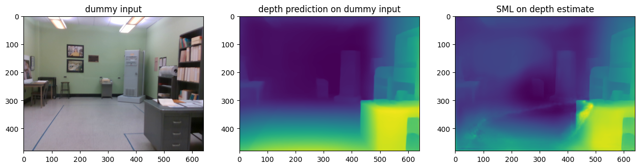
得られたダミー結果の保存と視覚化
# Base directory in which outputs would be stored as a pathlib.Path variable
OUTPUT_DIR = Path('output')

# Create the output directory adjacent to the notebook and suppress errors if the directory already exists
OUTPUT_DIR.mkdir(exist_ok=True)

# Utility functions are directly available in modules.midas.utils
# Provide path names without any extension and let the write_depth
# function provide them for you. Take note of the arguments.
utils.write_depth(path=str(OUTPUT_DIR / 'dummy_input'), depth=d_depth, bits=2)
utils.write_depth(path=str(OUTPUT_DIR / 'dummy_input_sml'), depth=sml_pred_dummy, bits=2)
plt.figure()

img_dummy_in = mpimg.imread('data/image/dummy_img.png')
img_dummy_out = mpimg.imread(OUTPUT_DIR / 'dummy_input.png')
img_dummy_sml_out = mpimg.imread(OUTPUT_DIR / 'dummy_input_sml.png')

f, axes = plt.subplots(1, 3)
plt.subplots_adjust(right=2.0)

axes[0].imshow(img_dummy_in)
axes[1].imshow(img_dummy_out)
axes[2].imshow(img_dummy_sml_out)

axes[0].set_title('dummy input')
axes[1].set_title('depth prediction on dummy input')
axes[2].set_title('SML on depth estimate')
Text(0.5, 1.0, 'SML on depth estimate')
<Figure size 640x480 with 0 Axes>
テスト画像で推論を実行
これで、ダミー入力、つまりダミー画像とそれに関連付けられた深度マップの両方の役割は終了です。コンパイルされたモデルにアクセスできるようになったため、純粋な推論目的で利用可能な 1 つの画像をロードし、深度マップのプロットまで上記のすべての手順を 1 つずつ実行できます。
このチュートリアルのデータ・ディレクトリーは次のように配置されています。これにより、これらの規則を遵守できます。
data
├── image
│   ├── dummy_img.png       # RGB images
│   └── <timestamp>.png
└── sparse_depth
    ├── dummy_img.png       # sparse metric depth maps
    └── <timestamp>.png     # as 16b PNG files
同時に、VOID データセットで使用される深度保存方法が想定されます。
画像のファイル名の形式を推測向けに考えている場合、その理由は次のとおりです。
データセットは、インテル® RealSense D435i カメラで収集されました。このカメラは、400 Hz で同期された加速度計とジャイロスコープ測定と、30 Hz で同期された VGA サイズ (640 x 480) RGB および深度ストリームを生成するように構成されています。深度フレームはアクティブステレオを使用して取得され、センサーの工場調整を使用して RGB フレームに揃えられます。センサーと深度ストリーム入力の頻度は一定の固定周波数で実行されるため、キャプチャーされたすべてのフレームにタイムスタンプを付けると、構造を維持するだけでなく、後でデバッグする際にも役立ちます。
推論の画像とそのスパース深度マップは、ここにある圧縮データセットから取得されます。
# As before download the sample images for inference and take note of the image hashes if you
# want to use them later
download_file('https://user-images.githubusercontent.com/22426058/254174393-fc6dcc5f-f677-4618-b2ef-22e8e5cb1ebe.png', filename='1552097950.2672.png', directory=Path(DATA_DIR / 'image'), silent=True)
download_file('https://user-images.githubusercontent.com/22426058/254174379-5d00b66b-57b4-4e96-91e9-36ef15ec5a0a.png', filename='1552097950.2672.png', directory=Path(DATA_DIR / 'sparse_depth'), silent=True)

# Load the image and its depth scale
img_input = data_loader.load_input_image('data/image/1552097950.2672.png')
img_depth_input = data_loader.load_sparse_depth('data/sparse_depth/1552097950.2672.png')

# Transform the input image for the depth model
transformed_image = transform_image_for_depth(input_image=img_input, depth_model_transform=depth_model_transform)

# Run the depth model on the transformed input
depth_pred = run_depth_model(input_image_h=IMAGE_H, input_image_w=IMAGE_W,
                             transformed_image=transformed_image, compiled_depth_model=compiled_depth_model)


# Call the function on the sparse depth map
# with all default settings and store in appropriate variables
int_depth, int_scales = compute_global_scale_and_shift(input_sparse_depth=img_depth_input, validity_map=None, depth_pred=depth_pred)

# Transform the input image for the ScaleMapLearner model
transformed_image_scale = transform_image_for_depth_scale(input_image=img_input,
                                                          scale_map_learner_transform=scale_map_learner_transform,
                                                          int_depth=int_depth, int_scales=int_scales)

# Run the SML model using the set of inputs
sml_pred = run_depth_scale_model(input_image_h=IMAGE_H, input_image_w=IMAGE_W,
                                 transformed_image_for_depth_scale=transformed_image_scale,
                                 compiled_scale_map_learner=compiled_scale_map_learner)
data/image/1552097950.2672.png: 0%| | 0.00/371k [00:00<?, ?B/s]
data/sparse_depth/1552097950.2672.png: 0%| | 0.00/3.07k [00:00<?, ?B/s]
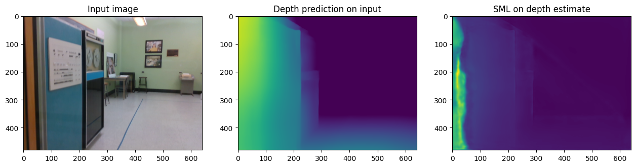
推論結果を保存して視覚化
# Store the depth and SML predictions
utils.write_depth(path=str(OUTPUT_DIR / '1552097950.2672'), depth=int_depth, bits=2)
utils.write_depth(path=str(OUTPUT_DIR / '1552097950.2672_sml'), depth=sml_pred, bits=2)


# Display result
plt.figure()

img_in = mpimg.imread('data/image/1552097950.2672.png')
img_out = mpimg.imread(OUTPUT_DIR / '1552097950.2672.png')
img_sml_out = mpimg.imread(OUTPUT_DIR / '1552097950.2672_sml.png')

f, axes = plt.subplots(1, 3)
plt.subplots_adjust(right=2.0)

axes[0].imshow(img_in)
axes[1].imshow(img_out)
axes[2].imshow(img_sml_out)

axes[0].set_title('Input image')
axes[1].set_title('Depth prediction on input')
axes[2].set_title('SML on depth estimate')
Text(0.5, 1.0, 'SML on depth estimate')
<Figure size 640x480 with 0 Axes>
データ・ディレクトリーのクリーンアップ
別のリポジトリーから画像と深度マップをダウンロードしたディレクトリーについても、同様に行います。ダウンロード・プロセス中に作成された不要なディレクトリーとファイルを削除します。
# Remove the data directory and suppress errors(if any)
rmtree(path=str(DATA_DIR), ignore_errors=True)
結論
このチュートリアルのコードは、VI-Depth リポジトリーを採用したものです。
ユーザーは、VOID データセットから元のデータセットと生のデータセットをダウンロードすることを選択できます。
isl-org/VI-Depth は、MiDaS 兄弟リポジトリーからリリースされたモデルアセットの少し古いバージョンで動作します。ただし、v3.1 以降の新しいリリースでは、OpenVINO™
.xmlおよび.binモデルファイルがアセットとして直接含まれるため、主要な前処理およびモデルコンパイルの手順は不要になります。