ImageBind と OpenVINO を使用したマルチモーダル・データのバインド

この Jupyter ノートブックは、ローカルへのインストール後にのみ起動できます。

周囲の世界を探索するとき、人々は、にぎやかな通りを見たり、車のエンジン音を聞いたりするなど、複数の感覚から情報を得ます。ImageBind は、さまざまな形式の情報から同時に、総合的に、直接的に学習する人間の能力にマシンを一歩近づけるアプローチを導入します。ImageBind は、明示的な監視 (生データを整理してラベル付けするプロセス) を必要とせずに、6 つのモダリティーからのデータを一度にバインドできる最初の AI モデルです。この画期的な技術は、画像とビデオ、音声、テキスト、深度、熱、慣性計測装置 (IMU) などのモダリティー間の関係を認識することで、マシンがさまざまな形式の情報をより適切に分析できるようにし、AI の進歩に貢献します。

ImageBind

このチュートリアルでは、OpenVINO を使用して ImageBind モデルを変換して実行する方法について説明します。

このチュートリアルは次のステップで構成されます。

1. 事前トレーニングされたモデルをダウンロードします。

2. 入力データの例を準備します。

3. モデルを OpenVINO 中間表現形式 (IR) に変換します。

4. モデル推論を実行し、結果を分析します。

ImageBind について

2023 年 5 月に Meta Research によってリリースされた ImageBind は、画像とビデオ、テキスト、オーディオ、熱画像、深度、加速度計や方向モニターなどのセンサーを含む IMU の 6 つのモダリティーからのデータを組み合わせる埋め込みモデルです。ImageBind を使用すると、オーディオなどの 1 つのモダリティーでデータを提供して、ビデオや画像などのさまざまなモダリティーで関連するドキュメントを見つけることができます。

ImageBind はデータのペアを使用してトレーニングされました。各ペアは、ビデオを含む画像データを別のモダリティーにマッピングし、結合されたデータを使用して埋め込みモデルをトレーニングしました。ImageBind は、トレーニングに使用した画像データを使用して、さまざまなモダリティーの特徴を学習できることを発見しました。ImageBind からの注目すべき結論は、画像を別のモダリティーとペアリングし、その結果を同じ埋め込み空間で組み合わせるだけで、マルチモーダル埋め込みモデルを作成できることです。モデルの詳細については、モデル・リポジトリー、論文、Meta AI ブログ投稿をご覧ください。

すべての埋め込みモデルと同様に、ImageBind には、情報検索、ゼロショット分類、下流のタスク (画像生成など) の入力として ImageBind 表現によって作成された使用例など、多数の潜在的な使用例があります。下の画像に示されている潜在的な使用例の一部は次のとおりです。

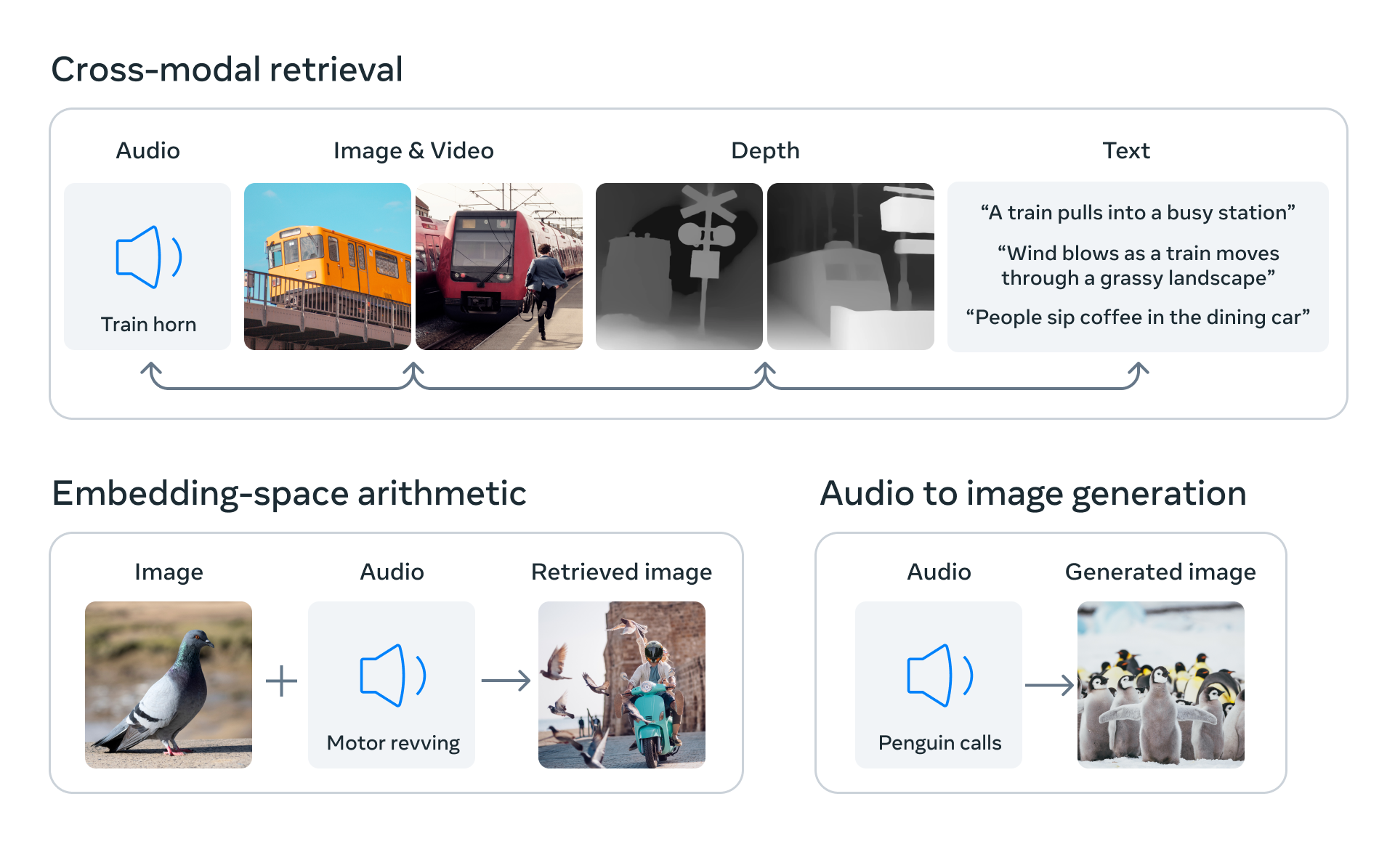
ユースケース

このチュートリアルでは、マルチモーダル・ゼロショット分類に ImageBind を使用する方法について説明します。

目次

• 必要条件

• PyTorch モデルをインスタンス化

• 入力データを準備

• モデルを OpenVINO 中間表現 (IR) 形式に変換

  • 推論デバイスの選択

• ImageBind と OpenVINO を使用したゼロショット分類

  • テキスト画像分類

  • テキスト音声分類

  • 画像音声の分類

• 次のステップ

必要条件

import sys

%pip install -q soundfile pytorchvideo ftfy "timm>=0.6.7" einops fvcore "openvino>=2023.1.0" numpy scipy matplotlib --extra-index-url https://download.pytorch.org/whl/cpu

if sys.version_info.minor < 8:
    %pip install -q "decord"
else:
    %pip install -q "eva-decord"

if sys.platform != "linux":
    %pip install -q "torch>=2.0.1" "torchvision>=0.15.2,<0.17.0" "torchaudio>=2.0.2"
else:
    %pip install -q "torch>=2.0.1" "torchvision>=0.15.2,<0.17.0" "torchaudio>=2.0.2" --index-url https://download.pytorch.org/whl/cpu

from pathlib import Path

repo_dir = Path("ImageBind")

if not repo_dir.exists():
    !git clone https://github.com/facebookresearch/ImageBind.git

%cd {repo_dir}

/home/ea/work/openvino_notebooks/notebooks/239-image-bind/ImageBind

PyTorch モデルをインスタンス化

モデルでの作業を開始するには、PyTorch モデルクラスをインスタンス化する必要があります。imagebind_model.imagebind_huge(pretrained=True) はモデルの重みをダウンロードし、ImageBind 用の PyTorch モデル・オブジェクトを作成します。現在、ダウンロード可能な ImageBind モデルは imagebind_huge のみです。詳細については、モデルカードをご覧ください。

インターネット接続速度によっては、モデルのダウンロード処理に時間がかかる場合があります。また、モデル・チェックポイントを保存するには、ディスク上に少なくとも 5 GB の空き容量が必要です。

import imagebind.data as data
import torch
from imagebind.models import imagebind_model
from imagebind.models.imagebind_model import ModalityType

# Instantiate model
model = imagebind_model.imagebind_huge(pretrained=True)
model.eval();

/home/ea/work/ov_venv/lib/python3.8/site-packages/torchvision/transforms/functional_tensor.py:5: UserWarning: The torchvision.transforms.functional_tensor module is deprecated in 0.15 and will be removed in 0.17. Please don't rely on it. You probably just need to use APIs in torchvision.transforms.functional or in torchvision.transforms.v2.functional.
  warnings.warn(
/home/ea/work/ov_venv/lib/python3.8/site-packages/torchvision/transforms/_functional_video.py:6: UserWarning: The 'torchvision.transforms._functional_video' module is deprecated since 0.12 and will be removed in the future. Please use the 'torchvision.transforms.functional' module instead.
  warnings.warn(
/home/ea/work/ov_venv/lib/python3.8/site-packages/torchvision/transforms/_transforms_video.py:22: UserWarning: The 'torchvision.transforms._transforms_video' module is deprecated since 0.12 and will be removed in the future. Please use the 'torchvision.transforms' module instead.
  warnings.warn(

入力データを準備

ImageBind は 6 つの異なるモダリティーにわたるデータを処理します。それぞれに前処理の手順が必要です。data モジュールは、各モダリティーのデータの読み取りと前処理を担当します。

• data.load_and_transform_text テキストラベルのリストを受け取り、トークン化します。

• data.load_and_transform_vision_data 入力画像へのパスを受け入れ、それを読み取り、小さい辺サイズ 224 でアスペクト比を保存するようにサイズを変更して、中央の切り取りを実行し、データを [0, 1] 浮動小数点範囲に正規化します。

• data.load_and_transofrm_audio_data 指定されたパスからオーディオファイルを読み取り、サンプルごとに分割し、メル・スペクトログラムを計算します。

# Prepare inputs

text_list = ["A car", "A bird", "A dog"]
image_paths = [".assets/dog_image.jpg", ".assets/car_image.jpg", ".assets/bird_image.jpg"]
audio_paths = [".assets/dog_audio.wav", ".assets/bird_audio.wav", ".assets/car_audio.wav"]

inputs = {
    ModalityType.TEXT: data.load_and_transform_text(text_list, "cpu"),
    ModalityType.VISION: data.load_and_transform_vision_data(image_paths, "cpu"),
    ModalityType.AUDIO: data.load_and_transform_audio_data(audio_paths, "cpu"),
}

モデルを OpenVINO 中間表現 (IR) 形式に変換

OpenVINO は、モデル変換 API を通じて PyTorch をサポートします。モデルを IR 形式に変換するには、モデル変換 Python API を使用します。ov.convert_model 関数は、デバイスにロードする準備が整った OpenVINO モデル・クラス・インスタンスを返すか、ov.save_model を使用して次回ロードするためにディスクに保存します。

ImageBind は、さまざまなモダリティーを同時に任意の組み合わせで表すデータを受け入れますが、それらの処理は互いに独立しています。データの受け渡しの柔軟性が失われないよう、各モダリティー・エンコーダーを独立したモデルとしてエクスポートします。以下のコードは、単一モダリティーの埋め込みのみを取得するためのモデルのラッパーを定義します。

class ModelExporter(torch.nn.Module):
    def __init__(self, model, modality):
        super().__init__()
        self.model = model
        self.modality = modality

    def forward(self, data):
        return self.model({self.modality: data})

import openvino as ov

core = ov.Core()

OpenVINO を使用して推論を実行するためにドロップダウン・リストからデバイスを選択します。

import ipywidgets as widgets

device = widgets.Dropdown(
    options=core.available_devices + ["AUTO"],
    value='AUTO',
    description='Device:',
    disabled=False,
)

device

Dropdown(description='Device:', index=2, options=('CPU', 'GPU', 'AUTO'), value='AUTO')

ov_modality_models = {}

modalities = [ModalityType.TEXT, ModalityType.VISION, ModalityType.AUDIO]
for modality in modalities:
    export_dir = Path(f"image-bind-{modality}")
    file_name = f"image-bind-{modality}"
    export_dir.mkdir(exist_ok=True)
    ir_path = export_dir / f"{file_name}.xml"
    if not ir_path.exists():
        exportable_model = ModelExporter(model, modality)
        model_input = inputs[modality]
        ov_model = ov.convert_model(exportable_model, example_input=model_input)
        ov.save_model(ov_model, ir_path)
    else:
        ov_model = core.read_model(ir_path)
    ov_modality_models[modality] = core.compile_model(ov_model, device.value)

INFO:nncf:NNCF initialized successfully. Supported frameworks detected: torch, tensorflow, onnx, openvino

No CUDA runtime is found, using CUDA_HOME='/usr/local/cuda'
/home/ea/work/openvino_notebooks/notebooks/239-image-bind/ImageBind/imagebind/models/multimodal_preprocessors.py:433: TracerWarning: Converting a tensor to a Python boolean might cause the trace to be incorrect. We can't record the data flow of Python values, so this value will be treated as a constant in the future. This means that the trace might not generalize to other inputs!
    if x.shape[self.time_dim] == 1:
/home/ea/work/openvino_notebooks/notebooks/239-image-bind/ImageBind/imagebind/models/multimodal_preprocessors.py:259: TracerWarning: Converting a tensor to a Python boolean might cause the trace to be incorrect. We can't record the data flow of Python values, so this value will be treated as a constant in the future. This means that the trace might not generalize to other inputs!
    assert tokens.shape[2] == self.embed_dim
/home/ea/work/openvino_notebooks/notebooks/239-image-bind/ImageBind/imagebind/models/multimodal_preprocessors.py:74: TracerWarning: Converting a tensor to a Python boolean might cause the trace to be incorrect. We can't record the data flow of Python values, so this value will be treated as a constant in the future. This means that the trace might not generalize to other inputs!
    if npatch_per_img == N:

ImageBind と OpenVINO を使用したゼロショット分類

ゼロショット分類では、データの一部が埋め込まれ、モデルに入力されて、データの内容に対応するラベルが取得されます。ImageBind では、音声、画像、その他のサポートされているモダリティーの情報を分類できます。CLIP モデルを使用してゼロショット画像分類を実行する方法についてはすでに説明しました (詳細についてはこのノートブックを確認してください)。ImageBind では、サポートされているモダリティーの任意の組み合わせを分類に使用できるため、このタスクに対する ImageBind の機能はより広範囲にわたります。

ImageBind を使用してゼロショット分類を実行するには、次の手順を実行する必要があります。

1. 要求されたモダリティーのデータバッチを前処理します (この場合、1 つのモダリティーはデータソースとして扱われ、他のモダリティーはラベルとして扱われます)。

2. 各モダリティーの埋め込みを計算します。

3. 埋め込みベクトル間のドット積を求めて確率行列を取得します。

4. ソースをラベル空間にマッピングするため最も高い確率を持つラベルを取得します。

前のステップですでにデータを前処理したので、埋め込みを取得するためにモデル推論を実行する必要があります。

embeddings = {}
for modality in modalities:
    embeddings[modality] = ov_modality_models[modality](inputs[modality])[ov_modality_models[modality].output(0)]

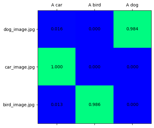
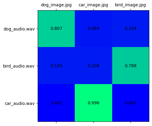
確率行列は、ソース埋め込みとラベル埋め込みの対応を示します。これは 2D 行列であり、x 次元はラベル・モダリティー・データを表し、y 次元はソース・モダリティー・データを表します。これは埋め込みベクトル間のドット積として計算でき、softmax を使用して [0,1] の範囲に正規化できます。次に、x ラベルと y ラベルの交差部分のスコアが高くなると、それらが同じオブジェクトを表す信頼性が高くなります。

import matplotlib.pyplot as plt
import numpy as np
from scipy.special import softmax


def visualize_prob_matrix(matrix, x_label, y_label):
    fig, ax = plt.subplots()
    ax.matshow(matrix, cmap='winter')

    for (i, j), z in np.ndenumerate(matrix):
        ax.text(j, i, '{:0.3f}'.format(z), ha='center', va='center')
        ax.set_xticks(range(len(x_label)), x_label)
        ax.set_yticks(range(len(y_label)), y_label)

image_list = [img.split('/')[-1] for img in image_paths]
audio_list = [audio.split('/')[-1] for audio in audio_paths]

text_vision_scores = softmax(embeddings[ModalityType.VISION] @ embeddings[ModalityType.TEXT].T, axis=-1)

visualize_prob_matrix(text_vision_scores, text_list, image_list)

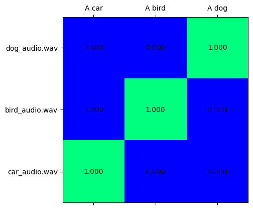
text_audio_scores = softmax(embeddings[ModalityType.AUDIO] @ embeddings[ModalityType.TEXT].T, axis=-1)

visualize_prob_matrix(text_audio_scores, text_list, audio_list)

audio_vision_scores = softmax(embeddings[ModalityType.VISION] @ embeddings[ModalityType.AUDIO].T, axis=-1)

visualize_prob_matrix(audio_vision_scores, image_list, audio_list)

これらすべてを組み合わせることで、データのテキスト、画像、音声を一致させることができます。

import IPython.display as ipd
from PIL import Image
text_image_ids = np.argmax(text_vision_scores, axis=0)
text_audio_ids = np.argmax(text_audio_scores, axis=0)
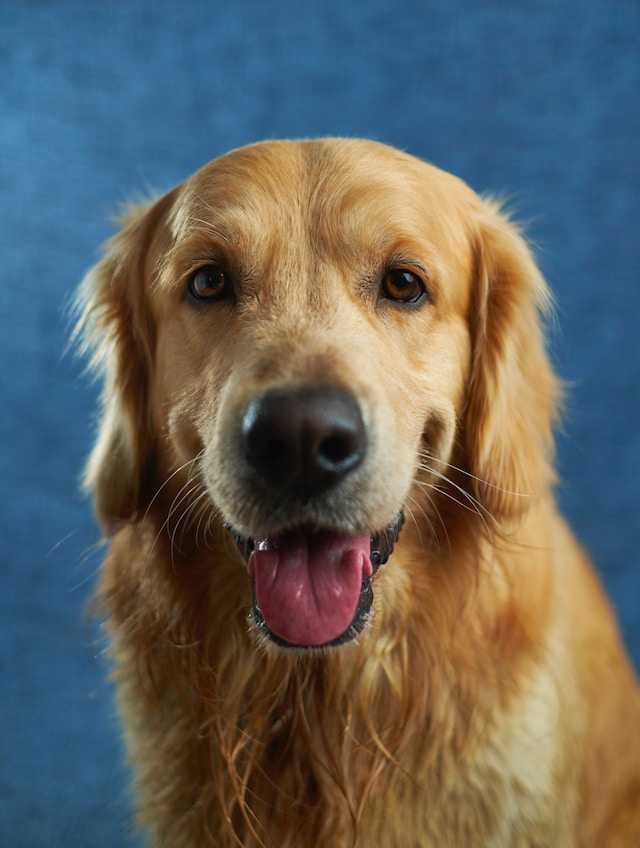
print(f"Predicted label: {text_list[0]} \nprobability for image - {text_vision_scores[text_image_ids[0], 0]:.3f}\nprobability for audio - {text_audio_scores[0, text_audio_ids[0]]:.3f}")
display(Image.open(image_paths[text_image_ids[0]]))
ipd.Audio(audio_paths[text_audio_ids[0]])

Predicted label: A car
probability for image - 1.000
probability for audio - 1.000

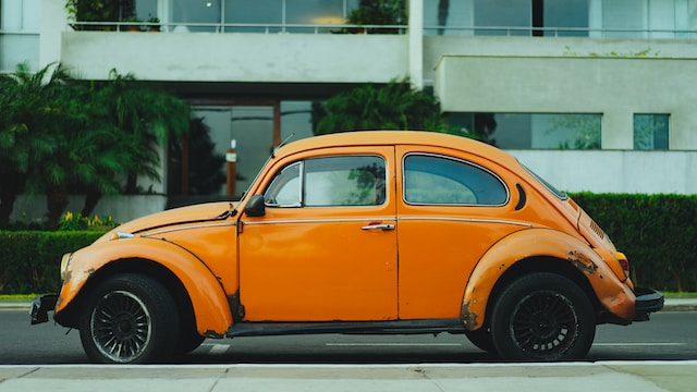
print(f"Predicted label: {text_list[1]} \nprobability for image - {text_vision_scores[text_image_ids[1], 1]:.3f}\nprobability for audio - {text_audio_scores[1, text_audio_ids[1]]:.3f}")
display(Image.open(image_paths[text_image_ids[1]]))
ipd.Audio(audio_paths[text_audio_ids[1]])

Predicted label: A bird
probability for image - 0.986
probability for audio - 1.000

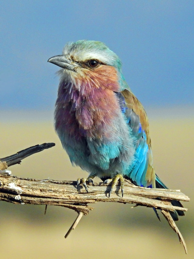
print(f"Predicted label: {text_list[2]} \nprobability for image - {text_vision_scores[text_image_ids[2], 2]:.3f}\nprobability for audio - {text_audio_scores[2, text_audio_ids[2]]:.3f}")
display(Image.open(image_paths[text_image_ids[2]]))
ipd.Audio(audio_paths[text_audio_ids[2]])

Predicted label: A dog
probability for image - 0.984
probability for audio - 1.000

次のステップ

239-image-bind-quantize ノートブックを開き、NNCF のトレーニング後の量子化 API を使用して IR モデルを量子化し、FP16 モデルと INT8 モデルを比較します。