Hello イメージのセグメント化

この Jupyter ノートブックはオンラインで起動でき、ブラウザーのウィンドウで対話型環境を開きます。ローカルにインストールすることもできます。次のオプションのいずれかを選択します。

OpenVINO™ でセグメント化モデルを使用する非常に基本的な入門編です。

このチュートリアルでは、Open Model Zoo の事前トレーニング済みの road-segmentation-adas-0001 モデルを使用します。ADAS は、Advanced Driver Assistance Services の略です。モデルは、背景、道路、縁石、マークの 4 つのクラスを認識します。

目次

• インポート

• モデルの重みをダウンロード

• 推論デバイスの選択

• モデルのロード

• 画像のロード

• 推論の実行

• 可視化のデータを準備

• データを可視化

# Install openvino package
%pip install -q "openvino>=2023.1.0"

Note: you may need to restart the kernel to use updated packages.

インポート

import cv2
import matplotlib.pyplot as plt
import numpy as np
import openvino as ov

# Fetch `notebook_utils` module
import urllib.request
urllib.request.urlretrieve(
                                        url='https://raw.githubusercontent.com/openvinotoolkit/openvino_notebooks/main/notebooks/utils/notebook_utils.py',
                                        filename='notebook_utils.py'
)

from notebook_utils import segmentation_map_to_image, download_file

モデルの重みをダウンロード

from pathlib import Path

base_model_dir = Path("./model").expanduser()

model_name = "road-segmentation-adas-0001"
model_xml_name = f'{model_name}.xml'
model_bin_name = f'{model_name}.bin'

model_xml_path = base_model_dir / model_xml_name

if not model_xml_path.exists():
                                        model_xml_url = "https://storage.openvinotoolkit.org/repositories/open_model_zoo/2023.0/models_bin/1/road-segmentation-adas-0001/FP32/road-segmentation-adas-0001.xml"
                                        model_bin_url = "https://storage.openvinotoolkit.org/repositories/open_model_zoo/2023.0/models_bin/1/road-segmentation-adas-0001/FP32/road-segmentation-adas-0001.bin"

                                        download_file(model_xml_url, model_xml_name, base_model_dir)
                                        download_file(model_bin_url, model_bin_name, base_model_dir)
else:
                                        print(f'{model_name} already downloaded to {base_model_dir}')

model/road-segmentation-adas-0001.xml:   0%|          | 0.00/389k [00:00<?, ?B/s]

model/road-segmentation-adas-0001.bin:   0%|          | 0.00/720k [00:00<?, ?B/s]

推論デバイスの選択

OpenVINO を使用して推論を実行するためにドロップダウン・リストからデバイスを選択します

import ipywidgets as widgets

core = ov.Core()
device = widgets.Dropdown(
                                        options=core.available_devices + ["AUTO"],
                                        value='AUTO',
                                        description='Device:',
                                        disabled=False,
)

device

Dropdown(description='Device:', index=1, options=('CPU', 'AUTO'), value='AUTO')

モデルのロード

core = ov.Core()

model = core.read_model(model=model_xml_path)
compiled_model = core.compile_model(model=model, device_name=device.value)

input_layer_ir = compiled_model.input(0)
output_layer_ir = compiled_model.output(0)

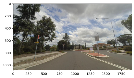
画像のロード

Mapillary Vistas データセットのサンプル画像が提供されています。

# Download the image from the openvino_notebooks storage
image_filename = download_file(
                                        "https://storage.openvinotoolkit.org/repositories/openvino_notebooks/data/data/image/empty_road_mapillary.jpg",
                                        directory="data"
)

# The segmentation network expects images in BGR format.
image = cv2.imread(str(image_filename))

rgb_image = cv2.cvtColor(image, cv2.COLOR_BGR2RGB)
image_h, image_w, _ = image.shape

# N,C,H,W = batch size, number of channels, height, width.
N, C, H, W = input_layer_ir.shape

# OpenCV resize expects the destination size as (width, height).
resized_image = cv2.resize(image, (W, H))

# Reshape to the network input shape.
input_image = np.expand_dims(
                                        resized_image.transpose(2, 0, 1), 0
)
plt.imshow(rgb_image)

data/empty_road_mapillary.jpg:   0%|          | 0.00/227k [00:00<?, ?B/s]

<matplotlib.image.AxesImage at 0x7f11c8142580>

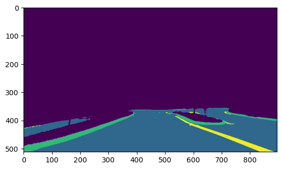
推論の実行

# Run the inference.
result = compiled_model([input_image])[output_layer_ir]

# Prepare data for visualization.
segmentation_mask = np.argmax(result, axis=1)
plt.imshow(segmentation_mask.transpose(1, 2, 0))

<matplotlib.image.AxesImage at 0x7f11c8051eb0>

可視化のデータを準備

# Define colormap, each color represents a class.
colormap = np.array([[68, 1, 84], [48, 103, 141], [53, 183, 120], [199, 216, 52]])

# Define the transparency of the segmentation mask on the photo.
alpha = 0.3

# Use function from notebook_utils.py to transform mask to an RGB image.
mask = segmentation_map_to_image(segmentation_mask, colormap)
resized_mask = cv2.resize(mask, (image_w, image_h))

# Create an image with mask.
image_with_mask = cv2.addWeighted(resized_mask, alpha, rgb_image, 1 - alpha, 0)

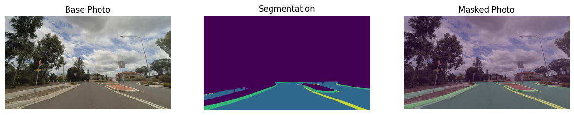
データを可視化

# Define titles with images.
data = {"Base Photo": rgb_image, "Segmentation": mask, "Masked Photo": image_with_mask}

# Create a subplot to visualize images.
fig, axs = plt.subplots(1, len(data.items()), figsize=(15, 10))

# Fill the subplot.
for ax, (name, image) in zip(axs, data.items()):
                                        ax.axis('off')
                                        ax.set_title(name)
                                        ax.imshow(image)

# Display an image.
plt.show(fig)